Using and Evaluating Logistic Regression in R
Introduction
What is Logistic Regression?
Imagine you're a bank trying to predict whether a loan applicant will default or not. You'd have several variables like income, credit score, and employment history. Logistic Regression helps you take all these variables into account to predict a 'Yes' or 'No'—will the applicant default?
You can also think of a similar example where you might want to recommend a product to a customer - is this customer likely to buy the product if they were recommended it?
What are we doing here?
You're going to import a popular dataset for this problem found here: https://archive.ics.uci.edu/dataset/144/statlog+german+credit+data
Getting Started: Laying the Groundwork
- Null Values: Data gaps can throw off our model, so we'll look for any missing information.
- Duplicates: Redundant data can skew results, so we'll eliminate any duplicates.
- Distributions: Understanding the shape of our data helps us know if any transformations are needed.
- Collinearity: Highly correlated variables can muddy our results, so we'll examine potential collinear relationships.
What We'll Cover:
- ROC (Receiver Operating Characteristic) Curve: To visualize the trade-offs between sensitivity and specificity.
- AUC (Area Under Curve): To summarize the model's performance in a single value.
- Basic Confusion Matrix: To give us a snapshot of how well our model is doing in terms of false positives, false negatives, etc.
Lets load the data
germancredit <- read.table("germancredit.txt", header=FALSE, sep=" ")
data <- germancredit
Rename Columns
new_names <- c("existing_checking_C",
"Duration_I",
"Credit_hist_C",
"Purpose_C",
"Cred_Amt_I",
"Savings_C",
"Employed_Dur_C",
"Rate_I",
"Status_Sex_C",
"Debt_C",
"Residence_I",
"Property_C",
"Age_I",
"Installment_Plans_C",
"Housing_C",
"Open_Credit_I",
"Job_C",
"Dependents_I",
"Telephone_B",
"International_Employee_B",
"Target")
colnames(data) <- new_names
Remove Duplicates (If any)
data <- unique(data)
Check for Nulls
null_count <- sapply(data, function(x) sum(is.na(x)))
print(paste("Null values by column: ", null_count))
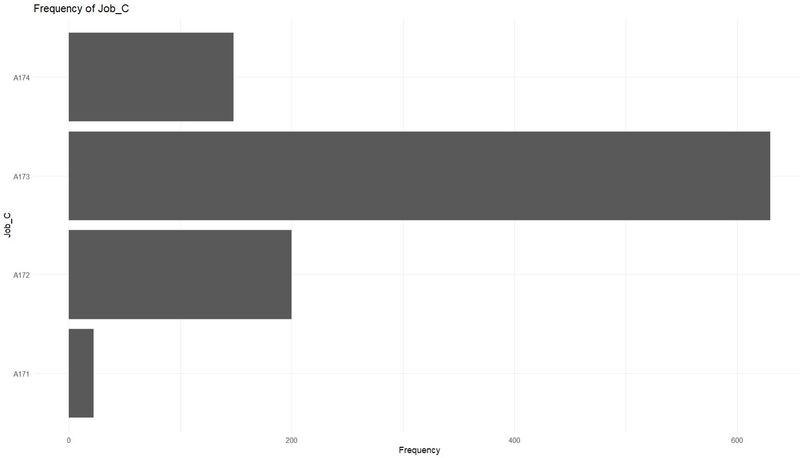
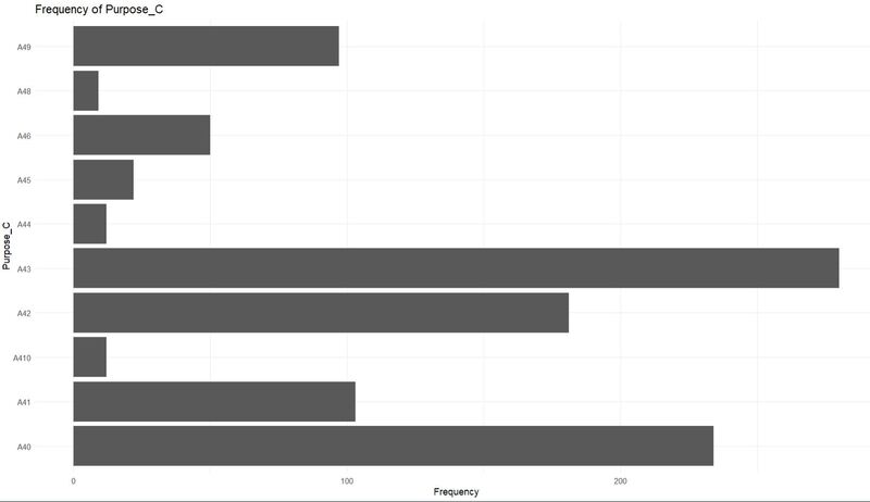
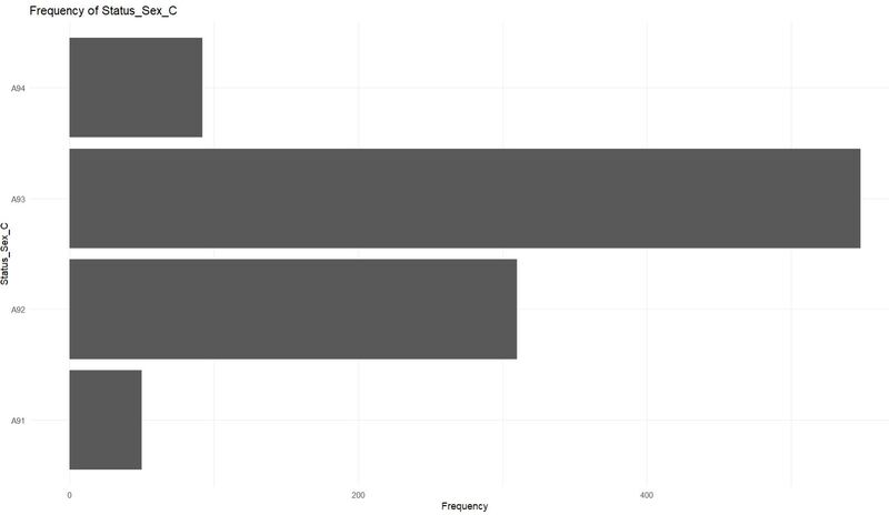
Exploratory Data Analysis (EDA) - Categorical Variables
library(ggplot2)
cat_cols <- grep("_C$", colnames(data), value = TRUE)
for(col in cat_cols) {
p <- ggplot(data, aes_string(col)) +
geom_bar() +
labs(title = paste("Frequency of", col), x = col, y = "Frequency") +
theme_minimal() +
coord_flip()
print(p)
}
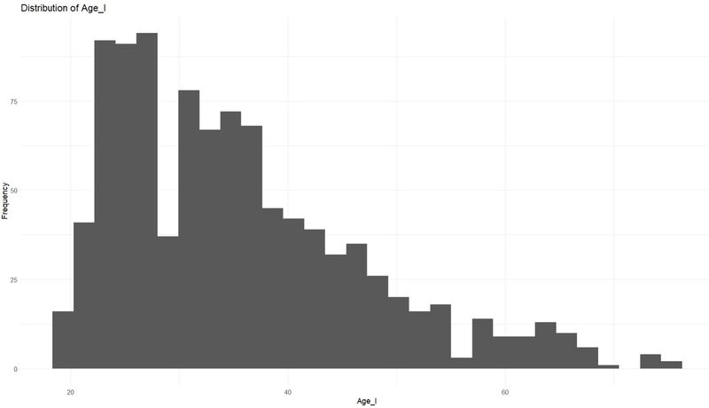
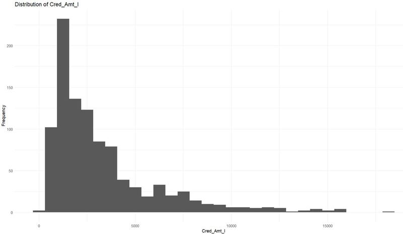
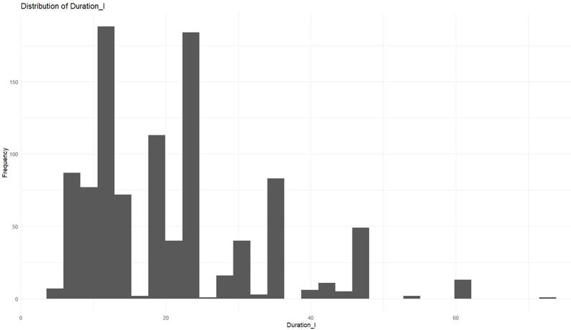
Exploratory Data Analysis (EDA) - Integer Variables
int_cols <- grep("_I$", colnames(data), value = TRUE)
for(col in int_cols) {
p <- ggplot(data, aes_string(col)) +
geom_histogram(bins=30) +
labs(title = paste("Distribution of", col), x = col, y = "Frequency") +
theme_minimal()
print(p)
}
Check for Collinearity
library(caret)
correlation_matrix <- cor(data[, int_cols], use = "pairwise.complete.obs")
highly_correlated <- findCorrelation(correlation_matrix, cutoff = 0.75)
print(paste("Columns with high collinearity: ", colnames(data)[highly_correlated]))
Encode Categorical Variables
The reason we do not numerically encode the variables is because this may introduce an issue where a feature labeled as "2" would be considered as 2x more than the feature labeled "1"
library(fastDummies)
data_encoded <- dummy_cols(data, select_columns = cat_cols, remove_first_dummy = TRUE, remove_selected_columns = TRUE)
For instance, imagine we have 3 categories, Red, Green, and Blue.
If our data is set up so that each category has a binary column telling us if there is a red, green, or blue color it would lead to a problem.
If we know that red and green are 0, we know for a fact that blue has to be 1.
Same goes for any other relationship with the colors. So if we remove one of the columns - we would still maintain all the information while removing an extraneous variable.
Update Binary Variables
First, let's confirm the data type and unique values for these columns.
levels(data_encoded$Telephone_B)
levels(data_encoded$International_Employee_B)
class(data_encoded$Telephone_B)
class(data_encoded$International_Employee_B)
unique(data_encoded$Telephone_B)
unique(data_encoded$International_Employee_B)
data_encoded$Telephone_B[data_encoded$Telephone_B == "A192"] <- 1
data_encoded$Telephone_B[data_encoded$Telephone_B == "A191"] <- 0
data_encoded$Telephone_B <- as.numeric(data_encoded$Telephone_B)
data_encoded$International_Employee_B[data_encoded$International_Employee_B == "A201"] <- 1
data_encoded$International_Employee_B[data_encoded$International_Employee_B == "A202"] <- 0
data_encoded$International_Employee_B <- as.numeric(data_encoded$International_Employee_B)
Update the Target Variable
data_encoded$Target <- data_encoded$Target - 1
Splitting the Data into Training and Validation
install.packages("caTools")
library(caTools)
set.seed(123) # Setting a seed for reproducibility
splitIndex <- sample.split(data_encoded$Target, SplitRatio = 0.7)
train_data <- data_encoded[splitIndex, ]
validation_data <- data_encoded[!splitIndex, ]
Building the Logistic Regression Model
logistic_model <- glm(Target ~ ., data = train_data, family = binomial)
summary(logistic_model)
While individual dummy variables might not be significant, the overall categorical variable can still be relevant.
Evaluating the Model
ROC CurveWe'll start by looking at the Receiver Operating Characteristic (ROC) curve, which is a graphical plot that illustrates the diagnostic ability of a binary classifier.
For this, we'll use the pROC package.
#install.packages("pROC")
library(pROC)
predicted_probs <- predict(logistic_model, newdata=validation_data, type="response")
roc_obj <- roc(validation_data$Target, predicted_probs)
plot(roc_obj, main="ROC Curve", col="#1c61b6", lwd=2)
abline(a=0, b=1, lty=2, col="gray") # Adding a reference line
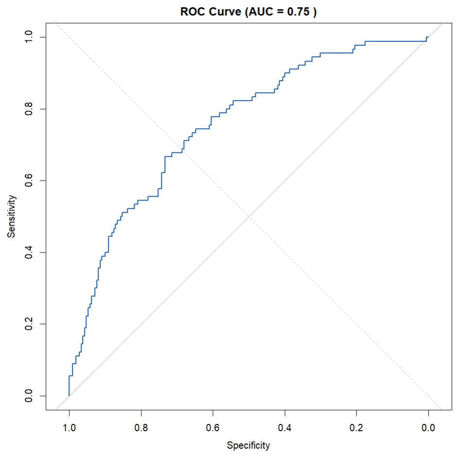
Understanding the ROC Curve
2. Ideal Curve: The most ideal ROC curve would hug the top-left corner. While our curve isn't perfect, it provides a starting point for understanding our model's performance.
3. Specificity & Sensitivity:
- When the curve is close to the bottom left (0,0) point, our model is conservative about classifying negatives. With a Specificity of 1, the model only identifies true negatives and avoids any false positives. But this also means Sensitivity is 0, and no true positives are identified.
- On the flip side, if Sensitivity is set to 1, the model will confidently label values as Positive only when there's absolutely no risk of them being negative. The same logic applies in reverse for Specificity.
4. Interpreting AUC: The AUC represents the area between the ROC curve and a 45-degree diagonal line (known as the line of no-discrimination). This diagonal line signifies a random classifier. A larger area indicates better model performance, while a smaller area suggests our model's performance is nearing random guessing.
5. Indentation in the Curve: The indentation seen in the middle of the curve indicates areas where the model finds it challenging to distinguish between the two classes. This could mean that within this range, both the positive and negative classes have similar probability scores.
6. Finding the Optimal Threshold: The optimal threshold is found at the point on the curve closest to the top-left corner. This point represents the optimal balance between Sensitivity and Specificity for our specific needs. Once we identify this point, we can then generate a confusion matrix to further understand the model's performance.
Extracting the ROC Coordinates
Youden's Index Explained: Youden's index is a statistic which can help to choose an optimal threshold that balances sensitivity and specificity in a way that the total performance is maximized. It is computed as: sensitivity + specificity - 1. The threshold at which the Youden's index is maximized is often considered as the optimal threshold. You can read more about it here:
https://en.wikipedia.org/wiki/Youden%27s_J_statistic
# Extracting the ROC Coordinates
full_coords <- coords(roc_obj, "all")
# You can access the roc_obj created to get the coordinates.
specificities <- full_coords$specificity
sensitivities <- full_coords$sensitivity
thresholds <- full_coords$threshold
# Calculating Youden's Index
youden_indices <- sensitivities + specificities - 1
# Finding and Plotting the Optimal Threshold
optimal_index <- which.max(youden_indices)
plot(1-specificities, sensitivities, type="l", xlim=c(0,1), ylim=c(0,1),
xlab="1-Specificity", ylab="Sensitivity", main="ROC Curve with Optimal Threshold")
points(1-specificities[optimal_index], sensitivities[optimal_index], col="red", pch=19, cex=1.5)
Note: This is NOT the optimal point for a model that relies on a cost solution.
In many business scenarios, you will need to look for some sort of assigned cost to getting a false positive or a false negative. Imagine if a bank is trying to determine whether or not someone is able to get a loan - if they aren't able to pay off that loan - then the bank loses money. So how many applicants should we deny that could have potentially been able to pay off a loan just so we can save on the costs of people who may potentially not pay off a loan.
Classifying Predictions Using the Optimal Threshold
# Extracting the Optimal Threshold
optimal_threshold <- thresholds[optimal_index]
# Classifying Predictions
predicted_classes <- ifelse(predicted_probs > optimal_threshold, 1, 0)
# Generating the Confusion Matrix
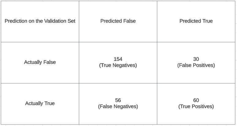
confusion_matrix <- table(predicted_classes, validation_data$Target)
# Displaying the Confusion Matrix
print(confusion_matrix)
Evaluating Classification Metrics
Confusion Matrix Breakdown:
- True Negatives (TN): The instances where the model correctly predicted the negative class.
- False Positives (FP): The instances where the model falsely predicted the positive class.
- False Negatives (FN): The instances where the model falsely predicted the negative class.
- True Positives (TP): The instances where the model correctly predicted the positive class.
Note: Note how I used the validation set. When we make models, we often test things on our validation set since the model was trained on the training set. The validation set is meant to act as "unseen" data so that you can evaluate the model's performance - sometimes another split called a "test" set is used as another layer of checking model performance.
# Given confusion matrix values
TN <- 154
FP <- 30
FN <- 56
TP <- 60
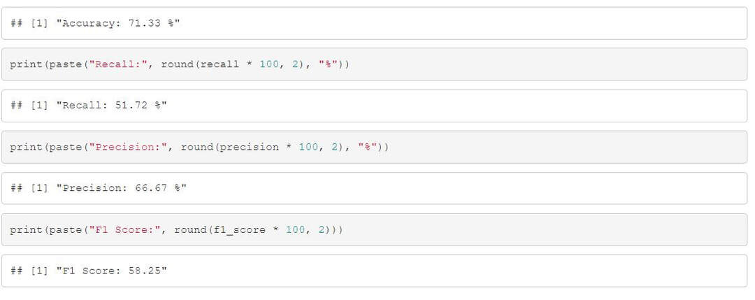
# Calculate Accuracy
accuracy <- (TP + TN) / (TP + TN + FP + FN)
print(paste("Accuracy:", accuracy))
# Calculate Precision
precision <- TP / (TP + FP)
print(paste("Precision:", precision))
# Calculate Recall
recall <- TP / (TP + FN)
print(paste("Recall:", recall))
# Calculate F1 Score
f1_score <- 2 * (precision * recall) / (precision + recall)
print(paste("F1 Score:", f1_score))
Assuming Costs Associated
Healthcare Diagnostics:
- Scenario: A CNN model is estimating if a tumor growth is benign or not in a patient's scans.
- Misclassification Costs:
- False Positive: Diagnosing a healthy person as having a tumor growth might lead to unnecessary treatments, stress, and medical costs. This can also lead to potential legal issues.
- False Negative: Failing to diagnose a sick person can lead to the progression of a disease, or more severe health complications
- Business Impact: Incorrect diagnoses can lead to increased medical costs, potential lawsuits, and a damaged reputation for the healthcare provider or diagnostic tool manufacturer.
This is exactly the kind of situation where getting many false positives or negatives is a pretty bad idea. You would probably look for a model with super high accuracy, but this isn't always the case. For this example, we might want to tailor a model to lean more heavily towards reducing the false negative rate. You might need to cast a wider net and overall have more false positives - and in this case it would be good because you'd be less likely to have a sick patient who wasn't captured by the model. You would want to increase recall and tailor the model around this. Accuracy is important - but we may need to trade off the other metrics as well.
In a case like the one below, we may consider a different approach.
E-commerce Fraud Detection:
- Scenario: E-commerce platforms employ fraud detection algorithms to identify potentially fraudulent transactions.
- Misclassification Costs:
- False Positive: If a legitimate transaction is flagged as fraudulent, the platform might decline the transaction or put it on hold, leading to an unhappy customer and potential loss of sales.
- False Negative: Failing to detect an actual fraudulent transaction can lead to financial losses, chargebacks, and increased processing fees.
- Business Impact: Not accurately detecting fraud can erode trust in the platform, lead to financial losses, and increase operational costs due to handling disputes and chargebacks.
In this case, we might want to make a model more focused on precision - and in doing so you would gain happier customers - but this does draw the risk of getting slightly more bad actors.
We are saying the cost of a False Positive is 1.1, and a False Negative is 1.2
FP_Cost = 1.1 # False Positive cost
FN_Cost = 1.2 # False Negative cost
threshold_seq <- seq(0, 1, 0.01)
costs_df <- data.frame(threshold = numeric(length(threshold_seq)),
cost = numeric(length(threshold_seq)),
class_0 = numeric(length(threshold_seq)),
class_1 = numeric(length(threshold_seq)),
TP = numeric(length(threshold_seq)),
TN = numeric(length(threshold_seq)),
FP = numeric(length(threshold_seq)),
FN = numeric(length(threshold_seq)))
We create a loop now that achieves this:
- Classify predictions based on the current threshold.
- Create a confusion matrix.
- Calculate the associated cost.
- Store results.
for (i in 1:length(threshold_seq)) {
threshold <- threshold_seq[i]
# DEBUG CHECK
print(paste("Processing threshold:", threshold))
# Step 2: Classify predictions based on the current threshold
predicted_classes <- ifelse(predicted_probs > threshold, 1, 0)
print(table(predicted_classes))
# Step 3: Create a confusion matrix
confusion_matrix <- table(Predicted = predicted_classes, Actual = validation_data$Target)
# We extract the results
# I needed to add this error check due to the error:
# "[.default`(confusion_matrix, 2, 1) : subscript out of bounds"
# This is because in some cases everything is a 1 or a 0 where the matrix doesn't have a corner to fill.
# This probably happens at extreme cases like 0.01 or .99
if (dim(confusion_matrix)[1] == 2 & dim(confusion_matrix)[2] == 2) {
TN <- confusion_matrix[1,1]
FP <- confusion_matrix[1,2]
FN <- confusion_matrix[2,1]
TP <- confusion_matrix[2,2]
} else {
# DEBUG STATEMENT
print(paste("Skipping threshold:", threshold, "due to non 2x2 confusion matrix"))
next # this will skip the current iteration of the loop
}
# We create our cost function
current_cost <- FN * FN_Cost + FP * FP_Cost
# DEBUG STATEMENT
print(paste("Cost at threshold", threshold, "is:", current_cost))
# Print the confusion matrix for each iteration:
rownames(confusion_matrix) <- c("Predicted 0", "Predicted 1")
colnames(confusion_matrix) <- c("Actual 0", "Actual 1")
print(confusion_matrix)
# Then we store our results in the empty dataframe, for each 'i'th value we store this in the dataframe.
costs_df[i, "threshold"] <- threshold_seq[i]
costs_df[i, "cost"] <- current_cost
costs_df[i, "class_0"] <- sum(predicted_classes == 0)
costs_df[i, "class_1"] <- sum(predicted_classes == 1)
costs_df[i, "TP"] <- TP
costs_df[i, "TN"] <- TN
costs_df[i, "FP"] <- FP
costs_df[i, "FN"] <- FN
# DEBUG STATEMENT
print(paste("Stored cost of", current_cost, "for threshold", threshold_seq[i], "at index", i))
}
costs_df <- costs_df[costs_df$threshold != 0.0, ]
After all thresholds are processed, we can find the one with the smallest cost.
min_cost_row <- costs_df[costs_df$cost == min(costs_df$cost), ]
optimal_threshold_cost <- min_cost_row$threshold
# the total costs for each threshold
plot(costs_df$threshold, costs_df$cost, type="l", xlab="Threshold", ylab="Total Cost", main="Total Cost for each Threshold")
abline(v=optimal_threshold_cost, col="red", lty=2)