- Published on
Clustering Hospitals
- Author
-
-
- Name
- Posts
- Posts
-

Hypothesis
Hospitals can be measured by minimum distances from each other. If the minimum distance between one hospital to another is large, we can assume that the area between them has a small population. At the same time, we can also assume if the distance between two hospitals is small, that area probably has a higher population. Like I mentioned before, hospitals are very expensive to construct and maintain, so it would make sense for hospitals to only be built where the general populace can benefit from it. If the minimum distance from one hospital to another hospital is 30 miles, then it can be safe to assume that there isn't enough of a population between these two hospitals to warrant building another. We are going to run with this theory, and create a map that clusters hospitals relative to the minimum distances they have from each other.
Let's get to work!
library(plyr)
library(lubridate)
library(ggplot2)
library(dplyr)
library(data.table)
library(ggrepel)
library(tidyverse)
library(ggmap)
#Installation for ggmap package here. Make sure you register your google api key with register_google(key = " ")
library(sp)
library(rgdal)
library(geosphere)
library(readxl)
library(matrixStats)
library(magick)
Note: You can still do this project in the same way if you prefer to use another dataset. Just make sure your dataset is comprehensive enough and has latitude and longitude points.
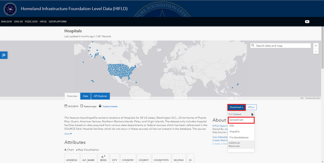
Going the distance
Hospitals <- read_csv("C:/Users/Daniel/Desktop/Hospitals.csv")
#If you are replicating this, make sure this goes to your file path
view(Hospitals)
x <- Hospitals$X
y <- Hospitals$Y
xy <- SpatialPointsDataFrame(
matrix(c(x,y), ncol = 2),
data.frame(ID = seq(1:length(x))),
proj4string=CRS("+proj=longlat +ellps=WGS84 +datum=WGS84"))
mdist <- distm(xy)
colnames(mdist) <- Hospitals$ADDRESS
rownames(mdist) <- Hospitals$ADDRESS
#What this does is create a spatial point data frame. To explain this simply, latitude and longitude coordinates are not plotted on a flat surface- the earth is round (this isn't a debate), so we are trying to look for the distance between 2 points, we need some sort of reference, which is the globe in this instance.
#we take the X values (longitude) and the Y values (latitude) from the dataset and make it a spatial points data frame.
#What we do after this is use the distm function to calculate the distance between each latitude and longitude. You can find out more about distm here
#distm(x, y ) takes the distance between x and y. If y is missing, it is the same as x. So since x in this case is the dataframe 'xy', I am finding the distance from every point to every other point in the xy dataframe.
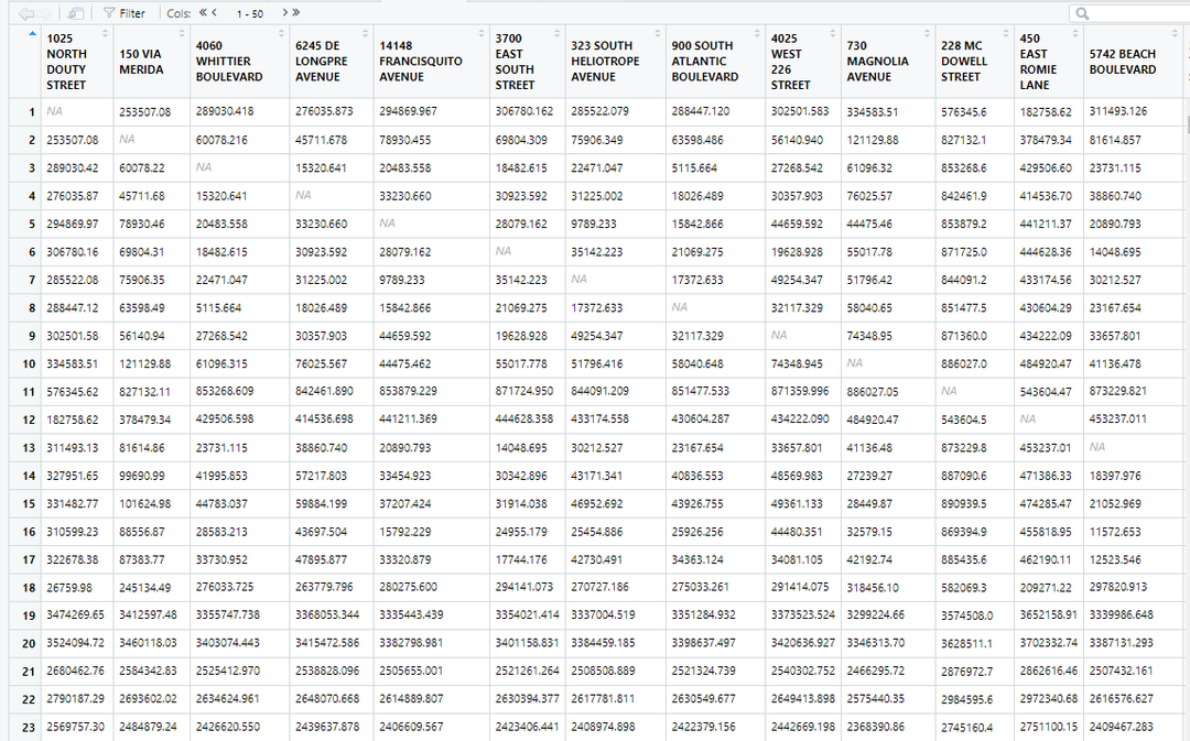
#Finally I name the rows and columns after the addresses of the hospitals. This gives me a table that looks like this:
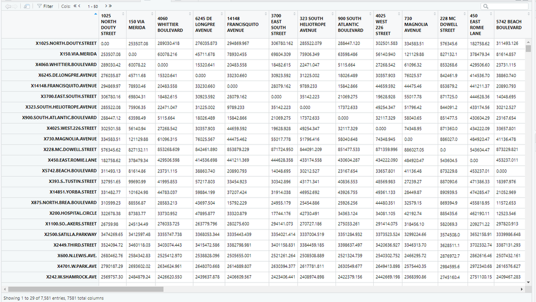
Each column and row name is a hospital. The entries that have a 0 value are a hospital's distance from itself! However, if I want to find the minimum distance to a different hospital, I will have to ignore 0. To do this, lets replace all 0 values with NA.
I am also aware that all the rows have their names strangely written compared to the columns. I only named the rows to explain how this distance dataset works, I will only need to use colnames() for the next step. So in the next pictures you'll see the rows go back to their original numerical values. You can keep or delete rownames() if you'd like, I will not be using it in the next steps.
mdist2 <- mdist
is.na(mdist2) <- mdist2==0
mdist3 <- rowMins(mdist2, na.rm = TRUE)
#view(mdist3)
mdist4 <- colnames(mdist2)[apply(mdist2,1,which.min)]
#view(mdist4)
Values <- c(1:7581)
Hospitals2 <- data.frame(Hospitals$X, Hospitals$Y, Hospitals$ADDRESS, Hospitals$NAME, Values, mdist3, mdist4, Hospitals$BEDS, Hospitals$TYPE,Hospitals$CITY,Hospitals$STATE,Hospitals$ZIP,Hospitals$STATUS)
names(Hospitals2) <- c("Longitude","Latitude","Address", "Name", "Values", "Distance","Closest_Address","BEDS","Type","City","State","ZIP","Status")
view(Hospitals2)
#mdist3 finds the minimum value of each row. However, I also want to know the column from which that value came from. So mdist4 uses which.min to tell me which column the minimum came from. You can find out how this is used in another example for maximum values here
#then I create a new dataset called Hospitals2. I use mdist3 and 4 and insert them into this dataset. Now I have a column that provides the closest hospital address, and also provides the distance to that hospital. Great! Now I am ready to cluster these hospitals relative to their distances.
Mapping
If you have the package, let's get started! A good place to familiarize yourself with ggmap is this excellent cheat sheet you can download here. You can also check out this blog for a great tutorial on ggmap.
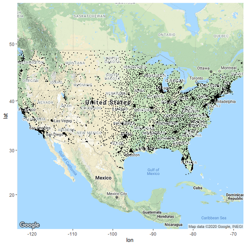
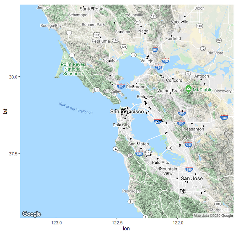
Lets just start off by plotting every hospital based on the latitude and longitude points.
p <- ggmap(get_googlemap(center = c("United States"),
zoom = 4, scale = 2,
maptype ='terrain',
color = 'color'))
p + geom_point(aes(x = Longitude, y = Latitude), data = Hospitals2, size = 0.5) +
theme(legend.position="bottom") +
windows()
#Notice how I used get_googlemap and then created a center called United States, which gets a map using google's service. Google recognizes that I want a map of the united states.
#You can use get_googlemap(center =c("")) just like you would go into google maps and search for a location.
If we want to sort the hospitals in relation to their distances, we need to set up some parameters for what these distances should be. I based my parameters from measuring the distances between various hospitals in the country from rural areas and urban areas. Remember; this is only a hypothesis and not meant to be exact.
Hospitals3 <- Hospitals2 %>% mutate(Classification = case_when(Distance >= 0 & Distance <= 300 ~ "Hospital Center",
Distance >= 300 & Distance <= 3000 ~ "Very Urban",
Distance >= 3001 & Distance <= 12000 ~ "Urban",
Distance >= 12001 & Distance <= 20000 ~ "Suburban",
Distance >= 20001 & Distance <= 30000 ~ "Rural",
Distance >= 30001 & Distance <= 300000 ~ "Very Rural"))
Hospitals_10_Urban <- filter(Hospitals3, Distance >= 0 & Distance <= 3000, BEDS >=0, Status == "OPEN")
Hospitals_8_Urban <- filter(Hospitals3, Distance >= 3001 & Distance <= 12000,BEDS >=0,Status == "OPEN")
Hospitals_6_Suburb <- filter(Hospitals3, Distance >= 12001 & Distance <= 20000,BEDS >=0,Status == "OPEN")
Hospitals_4_Rural <- filter(Hospitals3, Distance >= 20001 & Distance <= 30000,BEDS >=0,Status == "OPEN")
Hospitals_2_Very_Rural <- filter(Hospitals3, Distance >= 30001 & Distance <= 300000,BEDS >=0,Status == "OPEN")
#Distance is in meters. For now, I made all the hospitals under 300 meters into a "Hospital center". There are many hospitals within 300 meters of each other that are just part of the same hospital center . I will implement them later.
#Many Hospitals in the dataset have beds equal to -999. I assume it is an NA value. So I kept all hospitals with beds over 0.
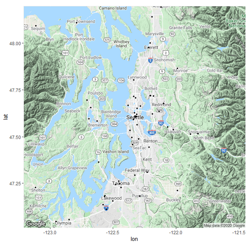
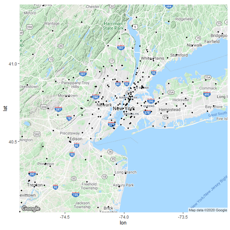
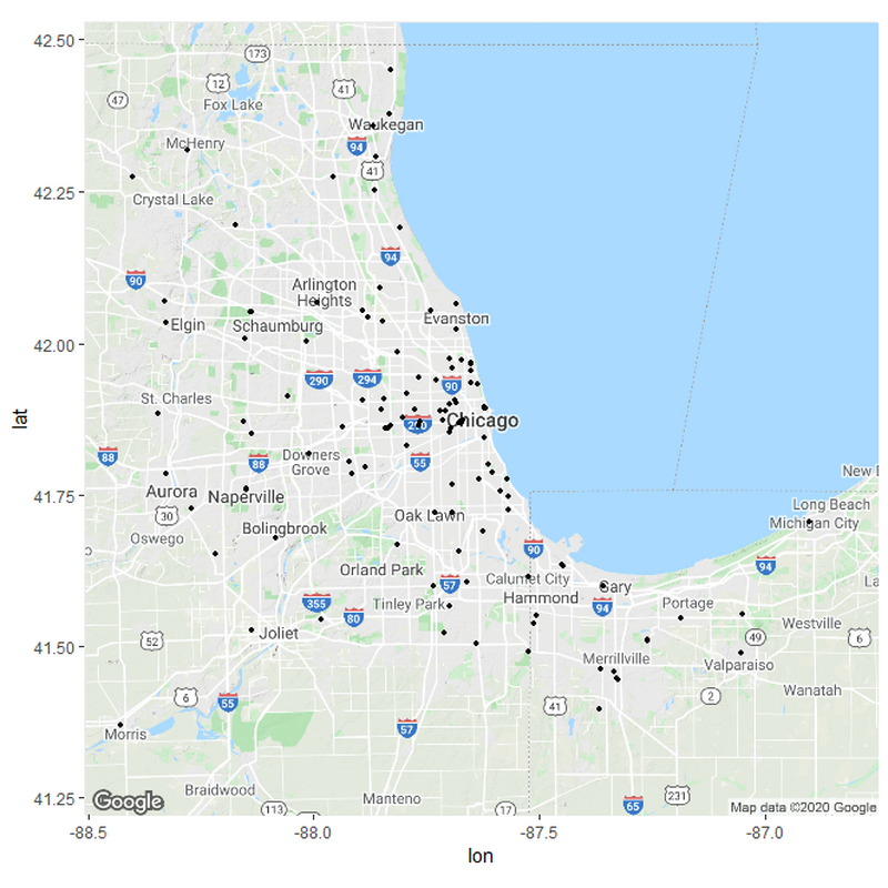
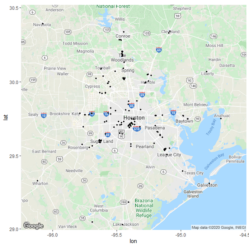
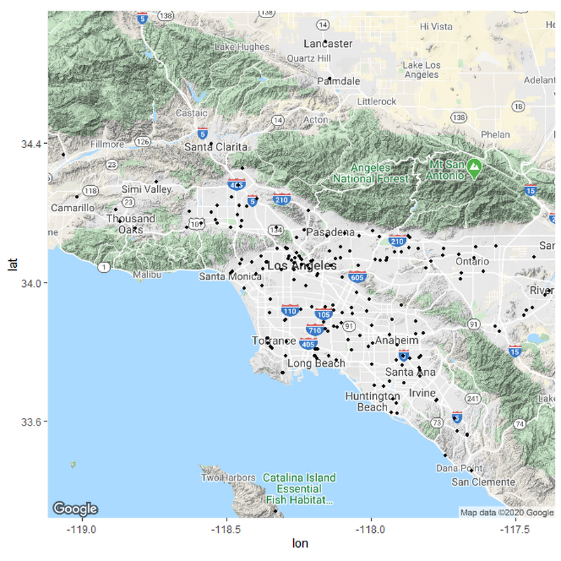
#Now we categorized each distance as a hypothetical scale for how urban an area is. We map this out and see how it looks like
m <- ggmap(get_googlemap(center = c("Insert Place Here"),
zoom = 8, scale = 2,
maptype ='roadmap',
color = 'color'))
m + geom_point(aes(x = Longitude, y = Latitude, size = BEDS, fill = Classification), pch = 21, data = Hospitals_10_Urban) +
geom_point(aes(x = Longitude, y = Latitude, size = BEDS,fill = Classification),pch = 21, data = Hospitals_8_Urban) +
geom_point(aes(x = Longitude, y = Latitude, size = BEDS,fill = Classification),pch = 21, data = Hospitals_6_Suburb) +
geom_point(aes(x = Longitude, y = Latitude, size = BEDS,fill = Classification),pch = 21, data = Hospitals_4_Rural) +
geom_point(aes(x = Longitude, y = Latitude, size = BEDS,fill = Classification),pch = 21, data = Hospitals_2_Very_Rural) +
theme(legend.position="right") +
labs(size = "Beds", fill = "Hypothesized Urbanicity")+
scale_fill_discrete(breaks=c("Hospital Center","Very Urban","Urban","Suburban","Rural","Very Rural"))+
scale_size(breaks = c(100,200,300,400,500,1000), range = c(1,6))+
windows()
#You can try out any area using ggmap and see how it clusters yourself.
However, since we have a distance matrix in mdist, we can take the lowest "n" values in each row, and average out the distances. That way, we could rely on "n" closest hospitals instead of just one.
mdistnew <- t(apply(mdist2, 1, sort))[, 1:5]
I only used the 5 smallest distances in this example, but you can try as many as you'd like by changing 5 in the above code to a higher number. Now all I do is create a new data frame using mdistnew.
colnames(mdistnew)[1:5]<- c("distance1","distance2","distance3","distance4","distance5")
#view(mdistnew)
mdistnew <- as.data.frame(mdistnew)
mdistnew$mean = (mdistnew$distance1+mdistnew$distance2+mdistnew$distance3+mdistnew$distance4+mdistnew$distance5)/5
Values <- c(1:7581)
Hospitals4 <- data.frame(Hospitals$X, Hospitals$Y, Hospitals$ADDRESS, Hospitals$NAME, Values, mdist3, mdist5, Hospitals$BEDS, Hospitals$TYPE,Hospitals$CITY,Hospitals$STATE,Hospitals$ZIP,Hospitals$STATUS,mdistnew)
names(Hospitals4) <- c("Longitude","Latitude","Address", "Name", "Values", "Distance","Closest_Address","BEDS","Type","City","State","ZIP","Status", "DistanceMinimum", "Distance2","Distance3","Distance4","Distance5","MeanDistance")
#view(Hospitals4)
#I used DistanceMinimum for simplicity, you can name the columns whatever you want
#mdistnew was converted to a dataframe so I could join it with other columns. If you do not convert it, you'll receive an error message.
#mdistnew$mean = ... creates a new column based off the mean of all distances. I basically added all the new distance columns and divided by the amount (5* in this case)
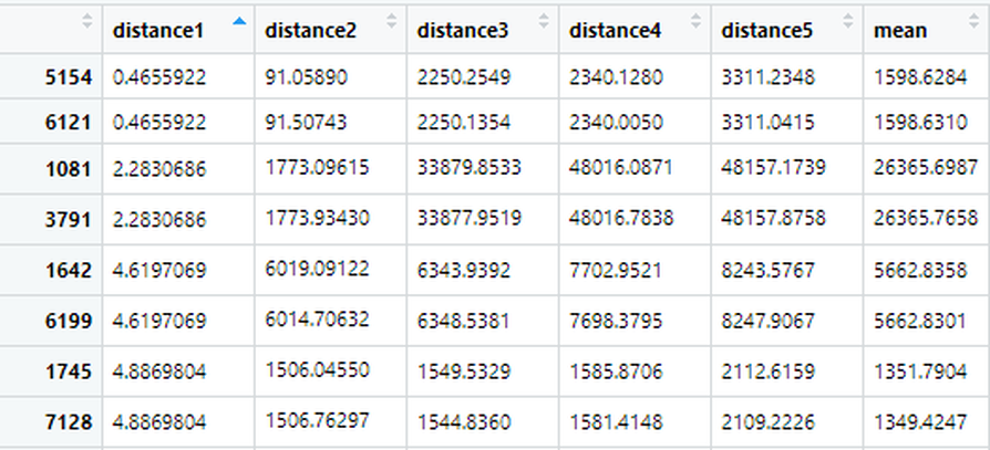
In this case, we now have 5 distances.If we check row 5154, the first 2 distances are only .4 and 90 meters from another hospital. Using the previous method, this hospital would be labeled as "Very Urban" or a "Hospital center". However, now we can use 5 distances to gauge just how close a hospital actually is from other hospitals in the area.
After looking at 5 distances in row 5154, we can say that the actual average distance to another hospital is around 1600 meters. This number can obviously change depending on how many distances we use.
Hospitals4 <- Hospitals4 %>% mutate(Classification = case_when(MeanDistance >= 0 & MeanDistance <= 3000 ~ "Very Urban",
MeanDistance >= 3001 & MeanDistance <= 12000 ~ "Urban",
MeanDistance >= 12001 & MeanDistance <= 20000 ~ "Suburban",
MeanDistance >= 20001 & MeanDistance <= 30000 ~ "Rural",
MeanDistance >= 30001 & MeanDistance <= 300000 ~ "Very Rural"))
#In the previous example, I labeled any hospitals with a minimum between 0 and 300 meters as "Hospital centers." Now we don't need to do that! We can comfortably go from 0 to 3000 meters (3km) without worrying about small distances skewing the cluster.
Hospitals_10_Urban <- filter(Hospitals4, MeanDistance >= 0 & MeanDistance <= 3000, BEDS >=0, Status == "OPEN")
Hospitals_8_Urban <- filter(Hospitals4, MeanDistance >= 3001 & MeanDistance <= 12000,BEDS >=0,Status == "OPEN")
Hospitals_6_Suburb <- filter(Hospitals4, MeanDistance >= 12001 & MeanDistance <= 20000,BEDS >=0,Status == "OPEN")
Hospitals_4_Rural <- filter(Hospitals4, MeanDistance >= 20001 & MeanDistance <= 30000,BEDS >=0,Status == "OPEN")
Hospitals_2_Very_Rural <- filter(Hospitals4, MeanDistance >= 30001 & MeanDistance <= 300000,BEDS >=0,Status == "OPEN")
#You can change the names that I used "Hospitals_10_Urban" to something else. I kept it the same throughout to make it easy to replicate this code.
#Now the parameters are based off an average.
z <- ggmap(get_googlemap(center = c(lon = -73.987086, lat = 40.745014),
zoom = 9, scale = 2,
maptype ='roadmap',
color = 'color'))
z + geom_point(aes(x = Longitude, y = Latitude, size = BEDS, fill = Classification), pch = 21, data = Hospitals_10_Urban) +
geom_point(aes(x = Longitude, y = Latitude, size = BEDS,fill = Classification),pch = 21, data = Hospitals_8_Urban) +
geom_point(aes(x = Longitude, y = Latitude, size = BEDS,fill = Classification),pch = 21, data = Hospitals_6_Suburb) +
geom_point(aes(x = Longitude, y = Latitude, size = BEDS,fill = Classification),pch = 21, data = Hospitals_4_Rural) +
geom_point(aes(x = Longitude, y = Latitude, size = BEDS,fill = Classification),pch = 21, data = Hospitals_2_Very_Rural) +
theme(legend.position="right") +
guides(fill = guide_legend(override.aes = list(size=10))) +
labs(size = "Beds", fill = "Hypothesized Urbanicity")+
scale_fill_discrete(breaks=c("Very Urban","Urban","Suburban","Rural","Very Rural"))+
scale_size(breaks = c(100,200,300,400,500,1000), range = c(1,6))+
windows()
#guides(fill = guide_legend(override.aes = list(size=10))) is a function to make the pch symbols in the legend larger. I find this really helpful for making legends visible
Updated Version
Old Version
z <- ggmap(get_googlemap(center = c("North West America"),
zoom = 7, scale = 2,
maptype ='roadmap',
color = 'color'))
z + geom_point(aes(x = Longitude, y = Latitude, size = BEDS, fill = Classification), pch = 21, data = Hospitals_10_Urban) +
geom_point(aes(x = Longitude, y = Latitude, size = BEDS,fill = Classification),pch = 21, data = Hospitals_8_Urban) +
geom_point(aes(x = Longitude, y = Latitude, size = BEDS,fill = Classification),pch = 21, data = Hospitals_6_Suburb) +
geom_point(aes(x = Longitude, y = Latitude, size = BEDS,fill = Classification),pch = 21, data = Hospitals_4_Rural) +
geom_point(aes(x = Longitude, y = Latitude, size = BEDS,fill = Classification),pch = 21, data = Hospitals_2_Very_Rural) +
theme(legend.position="right") +
guides(fill = guide_legend(override.aes = list(size=10))) +
labs(size = "Beds", fill = "Hypothesized Urbanicity")+
scale_fill_discrete(breaks=c("Very Urban","Urban","Suburban","Rural","Very Rural"))+
scale_size(breaks = c(100,200,300,400,500,1000), range = c(1,6))+
windows()